Preface
In the previous Costas Loop carrier-synchronization experiment we saw that, after symbol synchronization, the QPSK constellation first appears as a rotating ring, and the Costas Loop then corrects the frequency offset and phase until the ring converges into four stable clusters.
But how does the receiver pick the correct sampling position out of the several samples that fall inside every symbol? And when the transmit and receive sampling clocks disagree, how does it keep tracking the best sampling instant over time? These questions belong to symbol synchronization, also called timing recovery.
This article works through them.
Contents
Experimental environment and the receive chain
Why matched filtering alone is not enough for a hard decision
STO and SFO: why the sampling points drift
How the timing recovery loop finds the best sampling point
4.1 The interpolator: re-sampling between ADC samples
4.2 The timing error detector (TED): early or late?
4.3 The loop filter: smoothing the timing error
4.4 The NCO / timing control: where to sample next
5.Building and measuring the GNU Radio Symbol Sync block
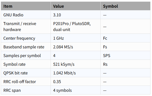
1. Experimental Environment and the Receive Chain
This article reuses the same transmit/receive bench as before, shown below:
Figure 1. The dual-P201Pro bench: transmit chain, wireless channel, receive chain and the GNU Radio flowgraph
Key parameters:
2. Why Matched Filtering Alone Is Not Enough
In the previous article (From Chaotic Constellations to QPSK Clusters: Costas Loop Carrier Synchronization, Measured) we introduced timing synchronization briefly, as a condition that has to be created before carrier synchronization can work. Here we go into how it actually works.
Start from the output of the matched filter. The corresponding GNU Radio flowgraph and the sink displays look like this:
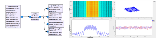
Figure 2. Signal after the matched filter only: sample rate is still 2.084 MS/s, four samples per symbol
Looking at the output on the right, the signal has only passed the matched filter so far; the sample rate is still 2.084 MS/s, and every symbol contains four samples:
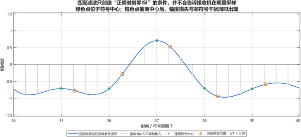
Figure 3. The continuous matched-filtered waveform with the 4-SPS input samples. Green dots mark the ideal symbol centers; the orange dots mark where the receiver actually samples right now (τ/T ≈ 0.28)
In the figure, green dots are the ideal symbol centers, and orange dots are the current, actual sampling positions. The goals of timing synchronization can be summarized as follows:
Find the best sampling instant inside each symbol period, so the sample lands as close as possible to the center of the eye, where inter-symbol interference (ISI) is smallest;
Compensate the initial timing offset, STO, so the receive sampling instants line up with the transmit symbol instants;
Continuously track the sampling-frequency offset, SFO, so the best sampling position does not slowly drift away as time passes — because the transmit and receive sampling clocks are not identical.
3. STO and SFO: Why the Sampling Points Drift
To isolate timing synchronization, ignore carrier frequency offset, phase offset and noise for now. After the channel and matched filter, the ideal sampling instant of the k-th symbol would be:
tk = kT
But the real receiver has an initial timing offset, and the two clocks are never exactly equal, so the actual sampling instant becomes:
tk = kT + τ0 + kΔT
where:
The total timing error of the k-th symbol is therefore:
τk = τ0 + kΔT
Here, τ0 is a fixed offset (the STO), while kΔT is the drift that SFO accumulates as the symbol index grows. In plain terms:
The whole picture is summarized in the figure below:
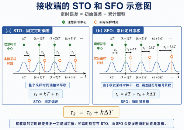
Figure 4. STO versus SFO at the receiver: (a) STO shifts the whole sampling timeline by a fixed τ0; (b) SFO makes the error grow by ΔT with every symbol: τk = τ0 + kΔT
4. How the Timing Recovery Loop Finds the Best Sampling Point
Section 3 gave us the receiver's timing error:
τk = τ0 + kΔT
where τ0 is the initial STO and kΔT is the timing drift accumulated by SFO over time.
If only STO existed, the receiver would, in theory, need to find the right sampling position once at start-up and then sample at a fixed symbol period forever. In practice, however, the transmitter and receiver use different clock sources, so the two sample rates can never be exactly equal. Even if you land on the best sampling position at the start, the sampling points will slowly creep away from the symbol center as time goes on.
In other words, timing synchronization is not "find the best point once and then keep sampling at fixed intervals". It must run as a continuously operating feedback loop:
detect the error → correct the sampling instant → detect again
This is the Timing Recovery Loop. In engineering terms, the classic interpolating timing recovery loop looks like this:
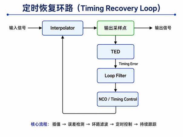
Figure 5. Structure of the interpolating timing recovery loop:Interpolator → output sample → TED → Loop Filter → NCO / Timing Control → back to the interpolator
The role of each block:
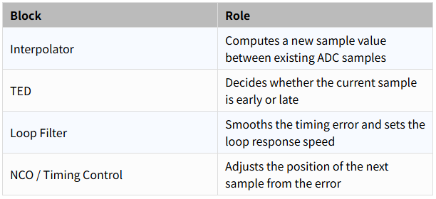
The loop repeats this cycle continuously, so the sampling position gradually converges toward the best symbol center and keeps tracking it even when SFO is present.
4.1 The Interpolator: Re-Sampling Between ADC Samples
Suppose the receiver currently has the ADC samples:
ADC samples:●--------●--------●--------●
↑
best sampling position
The best sampling position does not generally coincide with any single ADC sample. So you cannot simply:
4 SPS→take every 4th sample→1 SPS
Instead, the loop uses the nearby samples and interpolates the waveform value y(tk) at the target instant. Timing recovery is therefore not ordinary decimation: it is dynamically choosing where to sample, and interpolating that value.
4.2 The Timing Error Detector: Early or Late?
We now know the sampling position must be adjusted continuously. The remaining key question: how does the receiver tell whether the current sample is early or late? That is the job of the Timing Error Detector (TED). The TED produces a timing-error signal e[k] from the received waveform: the sign says which direction the sampling position must move, and the magnitude says how far off it is (the actual sign convention depends on the feedback direction of the loop).
Gardner is the classic TED for this job.
Gardner is a widely used timing error detector. It does not directly decide where to sample next; instead, it uses three samples belonging to two adjacent symbols to judge whether the current timing is early or late. Let the estimated centers of two adjacent symbols be t̂k−1 and t̂k, one symbol period T apart. The three Gardner samples are:
Ek = y(t̂k−1) — Early: the sample at the previous symbol center;
Mk = y(t̂k−1 + T/2) — Mid: the sample at the half-symbol point between the two centers;
Lk = y(t̂k) — Late: the sample at the current symbol center, which is also the symbol sample passed to later processing.
On the time axis they look like this:

For complex baseband signals, a common Gardner error expression is:
ek = Re { (Ek − Lk) · Mk* }
where Mk* is the complex conjugate of Mk and Re takes the real part. (Ek − Lk) describes the change between the samples at the two adjacent symbol centers, and Mk reflects the waveform state halfway between them. Combined, they reveal the direction of the current timing offset relative to the best sampling instant:
When the timing is early or late, the waveform is no longer symmetric about the half-symbol point, and ek comes out as a positive or negative value with a definite direction;
Once the loop is locked, the instantaneous error still fluctuates because of noise and data, but its long-term average should be close to zero:
E{ek} ≈ 0
Note that different references or software implementations may use the opposite error sign, so "positive means early" must be checked against the feedback direction of the specific loop. This does not change the principle: the error drives the interpolator and the sampling position converges toward the best instant.
4.3 The Loop Filter: Smoothing the Timing Error
The Gardner output e[k] contains noise and instantaneous fluctuations, so it cannot directly drive the sampling position. It must first pass through a loop filter:
e[k] → Loop Filter → u[k]
where u[k] is the smoothed timing control quantity. Just as with the Costas Loop discussed earlier, the loop bandwidth trades off two things:
Larger bandwidth → faster convergence, but more timing jitter;
Smaller bandwidth → smoother tracking, but slower convergence.
4.4 The NCO / Timing Control: Where to Sample Next
The control quantity after the loop filter must be converted into "where should we sample next". The NCO can be thought of as a continuously running timing reference. From the currently estimated symbol period and the loop correction, it decides the next interpolated sampling position:
t̂k+1 = t̂k + T̂ + u[k]
where t̂k is the current estimated sampling instant, T̂ is the current estimated symbol period, and u[k] is the correction produced by the timing loop.
One thing to notice: the NCO in carrier control adjusts phase; the NCO in timing control adjusts the sampling instant.
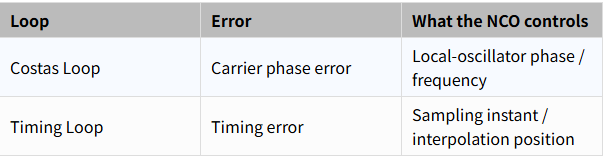
So in practice: Gardner tells you whether you are early or late, the loop filter decides how much to correct, and the NCO plus interpolator actually move the next sample there.
5. Building and Measuring the GNU Radio Symbol Sync Block
The interpolator, TED, loop filter and NCO described above are all packaged inside GNU Radio's Symbol Sync block:
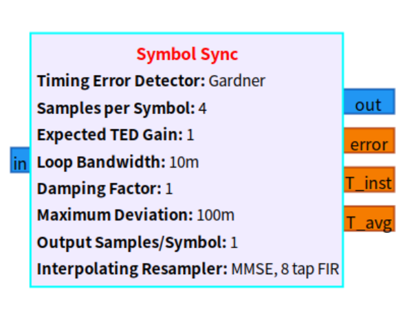
Figure 6. The GNU Radio Symbol Sync block and its parameters used in this experiment
Mapping the GNU Radio parameters to the theory:
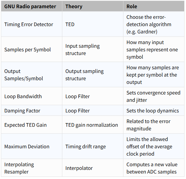
The block's position in the receiver is:
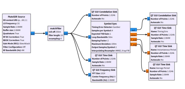
Figure 7. Symbol Sync sits right after the matched filter: 4 samples/symbol in, 1 sample/symbol out, with timing-loop monitors attached
Symbol Sync follows the matched filter. Its input keeps four samples per symbol, and its output keeps one sample per symbol. Running the flowgraph gives the results below:
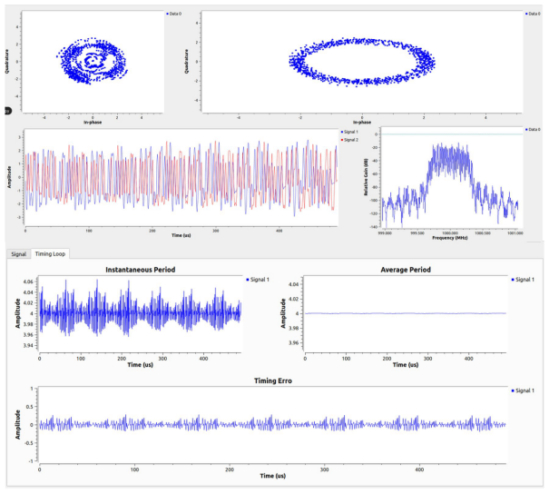
Figure 8. Measured results: constellation before (left, multi-layer scatter) versus after (right, a narrow rotating elliptical ring); timing-loop monitors — Instantaneous Period fluctuating around 4, Average Period settled at 4, Timing Error fluctuating around zero
From the constellation plot, the input samples before Symbol Sync form a multi-layer, messy scatter, while after synchronization the constellation clearly converges into a narrow rotating elliptical ring. The loop has selected a relatively stable decision sample out of the multiple input samples per symbol, and the samples taken during transition points are strongly suppressed. The constellation does not yet form four fixed clusters because the residual carrier frequency offset and phase offset still make the QPSK symbols rotate — that part is handed to the Costas Loop in the next article.
The three timing-loop monitors confirm the lock:
Instantaneous Period fluctuates around 4, showing the loop correcting the instantaneous sampling interval symbol by symbol;
Average Period settles long-term near 4, matching the configured 4 SPS — the estimated average symbol period is stable;
Timing Error fluctuates around zero with no one-sided drift — the current sampling position is being tracked steadily.
So you cannot judge symbol synchronization from the constellation forming a ring alone; you should read the instantaneous period, average period and timing error together. The current results show that Symbol Sync has entered a stable tracking state, and it hands a much steadier symbol-sample sequence to the Costas Loop carrier synchronization that follows.
Hardware: dual PZSDR P201Pro (AD9361, ±0.5 ppm VCTCXO), GNU Radio 3.10. Fc = 1 GHz, Fs = 2.084 MS/s, SPS = 4, Rs = 521 kSym/s, RRC roll-off 0.35.